Viewing the Results
Because ModelBuilder-2D incorporates the full ParaView visualization feature set, there are numerous ways to display the stress and displacement data computed by MinimalFEM After enabling the ParaView visualization features and loading the computed data, we will show three different ways to display the data.
18. Enable ParaView Features
By default, ModelBuilder-2D hides the ParaView pipeline inspector and related toolbars and filters. To see them, find and click the toolbar button with a gray ParaView icon. Once clicked, the button will change to display the familiar red-green-blue ParaView logo, a number of new toolbars will be displayed, and the Pipeline Browser view will display in the sidebar.

For convenience, undock the Pipeline Browser and drag it over the Attribute Editor view so that it is displayed as another tab.
19. Add a Third Layout and RenderView
Follow the same steps as before (Add a RenderView) to create a (third) RenderView tab:
In the tab bar above the current RenderView, click the + button.
In the new tab, click the Render View button.
Click the Camera Reset button to center the model and mesh contents.
Right click on the content and select Hide. You will need to do this twice to hide both the model and mesh respectively.
Right click on the new tab label and rename it “Results”.
20. Load the VTP Data
In the previous step (Running the MinimalFEM Solver) the results of the elasticity calculations were written to a minfem.vtp file under the project directory. Go to the File menu and select the Open… item, navigate to your project directory, then the export subdirectory, select the minfem.vtp file, and click the OK button. ModelBuilder will display a dialog titled Open Data With… listing a number of readers for VTK polydata files. Choose the XML PolyData Reader and click the OK button. ModelBuilder-2D will load the file and render a basic 2-D display. That display will show the computed stress values; because they are calculated on mesh elements, you can see faceting in the data.
To produce a smooth display, go to the Filters menu, open the Alphabetical submenu and select the Cell Data To Point Data item. This creates a new set of point data that can be interpolated by the graphics hardware.

21. Open the Properties View
The main visualization features can be accessed from the Properties view. To open this view, go to the View menu and check the box next to Properties. When the Properties view appears in the sidebar, you can undock it and drag it over the other tabbed views and dock it as another tab.
22. Add WarpByVector Filter
To visualize physical distortion, first go back to the original display settings - do this by going to the Pipeline Browser tab and use the eyeball icons to hide `CellDataToPointData1 and show minfem.vtp. Then select the minfem.vtp item, go to the Filters menu, select the Common submenu, and select Warp By Vector.
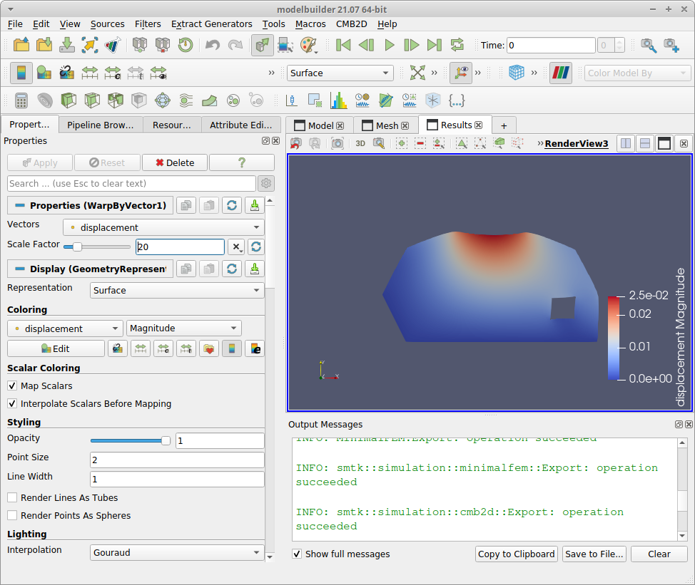
In the Properties tab, you will find three top-level sections labeld Properties (WarnByVector1), Display (GeometryRepresentation), and View (Render View). We suggest that you collapse all three sections and open them one at a time to make these changes.
In the first section – Properties (WarnByVector1)` – set the Scale Factor to
25.In the second section – Display (GeometryRepresentation) – set the Coloring to
displacement.
Note
After typing a numerical field in the Properties View, either hit the <Enter> key or click the Apply button to apply the change.
With these settings, you can see bowing of the upper edge and skewing of the hole geometry.
23. Add Glyph Filter
To display the strain field with vector arrows, go to the Pipeline Browser tab and:
hide the
WarpByVector1item,show the
CellDataToPointData1item,select the
minfem.vtpitem.
Then go to the Filters menu, select the Common submenu, and select Glyph. You will see some warning messages in the Output Messages view, which we will deal with next. (You can clear the Output Messages.)
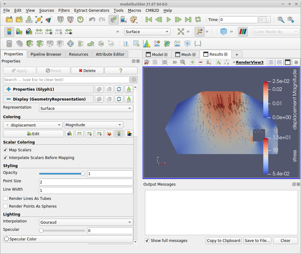
The Properties view now has three top-level sections labeled Properties (Glyph1), Display (GeometryRepresentation), and View (Render View). We suggest you collapse all three before setting the following properties:
Expand the Properties (Glyph1) section and
Find the Scale subsection and set Scale Array to
displacement.In the Scale subsection, set Scale Factor to
50.Find the Masking subsection and set the Maximum Number Of Sample Points to
400.Collapse the Properties (Glyph1) section.
Expand the Display (GeometryRepresentation) section and:
Find the Coloring subsection and set it to
displacement.
When you are done, you should see a set of arrow-shaped glyphs colored and scaled by the magnitude of computed displacement data, with the polygon colored by the computed stress data.
These examples should give you some idea of what you can do with ModelBuilder and the CMB platform. With the full range of ParaView` feature available, you can explore many more properties, filters, and other options.